But notice a subtle difference: This code deals
with the memory representation of a
tree, not the structure of the tree
itself. It treats the tree as consisting of cells, each containing some data
plus pointers to two more cells.
Visual
Prolog allows truly recursive type definitions in which the pointers are
created and maintained automatically. For example, you can define a tree as
follows:
DOMAINS
treetype = tree(string,
treetype, treetype)
This declaration says that a tree will be
written as the functor, tree, whose arguments are a string
and two more trees.
But this isn't quite right; it provides no way
to end the recursion, and, in real life, the tree does not go on forever. Some
cells don't have links to further trees. In Pascal, you could express this by
setting some pointers equal to the special value nil, but pointers are an
implementation issue that ordinarily doesn't surface in Prolog source code.
Rather, in Prolog we define two kinds of trees: ordinary ones and empty ones.
This is done by allowing a tree to have either of two functors: tree,
with three arguments, or empty, with no arguments.
DOMAINS
treetype = tree(string,
treetype, treetype) ; empty
Notice that the names tree (a functor that
takes three arguments) and empty (a functor taking no
arguments) are created by the programmer; neither of them has any pre-defined
meaning in Prolog. You could equally well have used xxx and yyy.
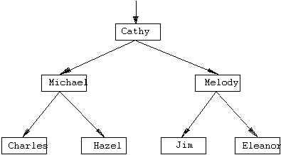
This is how the tree in Figure 6.1 could
appear in a Prolog program:
tree("Cathy",
tree("Michael"
tree("Charles",
empty, empty)
tree("Hazel",
empty, empty))
tree("Melody"
tree("Jim", empty,
empty)
tree("Eleanor",
empty, empty)))
This is indented here for readability, but
Prolog does not require indentation, nor are trees indented when you print them
out normally. Another way of setting up this same data structure is:
tree("Cathy"
tree("Michael", tree("Charles", empty, empty),
tree("Hazel", empty, empty))
tree("Melody", tree("Jim", empty, empty),
tree("Eleanor", empty, empty)))
Note that this is not a Prolog clause; it is
just a complex data structure.
(1) Traversing a Tree
Before
going on to the discussion of how to create trees, first consider what you'll
do with a tree once you have it. One of the most frequent tree operations is to
examine all the cells and process them in some way, either searching for a
particular value or collecting all the values. This is known as traversing the tree. One basic algorithm
for doing so is the following:
If the tree is empty, do nothing.
Otherwise, process the current node, then traverse the left subtree,
then traverse the right subtree.
Like the tree itself, the algorithm is
recursive: it treats the left and right subtrees exactly like the original
tree. Prolog expresses it with two clauses, one for empty and one for nonempty
trees:
traverse(empty).
/* do nothing */
traverse(tree(X, Y, Z)) :-
do something with X,
traverse(Y),
traverse(Z).

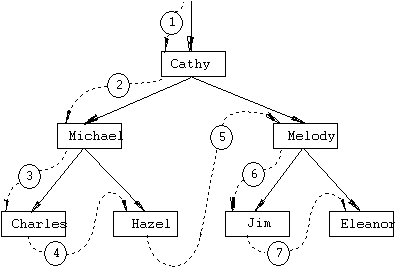
Figure 6.2: Depth-First Traversal of the Tree in
Figure 6.1
This tree traversal algorithm is known as depth-first search because it goes as
far as possible down each branch before backing up and trying another branch
(Figure 6.2). To see it in action,
look at program 9, which traverses a tree and prints all the elements as it
encounters them. Given the tree in Figures 6.1 and 6.2, 9 prints
Cathy
Michael
Charles
Hazel
Melody
Jim
Eleanor
Of course, you could easily adapt the program
to perform some other operation on the elements, rather than printing them.
/* Program ch06e09.pro */
/*
Traversing a tree by depth-first search
and printing each element as it is encountered */
DOMAINS
treetype = tree(string,
treetype, treetype) ; empty()
PREDICATES
traverse(treetype)
CLAUSES
traverse(empty).
traverse(tree(Name,Left,Right)):-
write(Name,'\n'),
traverse(Left),
traverse(Right).
GOAL
traverse(tree("Cathy",
tree("Michael",
tree("Charles", empty, empty),
tree("Hazel", empty, empty)),
tree("Melody",
tree("Jim", empty, empty),
tree("Eleanor",
empty, empty)))).
Depth-first search is strikingly similar to the
way Prolog searches a knowledge base, arranging the clauses into a tree and
pursuing each branch until a query fails. If you wanted to, you could describe
the tree by means of a set of Prolog clauses such as:
father_of("Cathy",
"Michael").
mother_of("Cathy",
"Melody").
father_of("Michael",
"Charles").
mother_of("Michael",
"Hazel").
...
This is preferable if the only purpose of the
tree is to express relationships between individuals. But this kind of
description makes it impossible to treat the whole tree as a single complex
data structure; as you'll see, complex data structures are very useful because
they simplify difficult computational tasks.
(2) Creating a Tree
One
way to create a tree is to write down a nested structure of functors and
arguments, as in the preceding example (Program 9). Ordinarily, however, Prolog
creates trees by computation. In each step, an empty subtree is replaced by a
nonempty one through Prolog's process of unification (argument matching).
Creating a one-cell tree from an ordinary data
item is trivial:
create_tree(N, tree(N,
empty, empty)).
This says: "If N is a data item, then tree(N, empty, empty) is a one-cell tree containing it."
Building a tree structure is almost as easy.
The following procedure takes three trees as arguments. It inserts the first
tree as the left subtree of the second tree, giving the third tree as the
result:
insert_left(X, tree(A, _,
B), tree(A, X, B)).
Notice that this rule has no body--there are no
explicit steps in executing it. All the computer has to do is match the
arguments with each other in the proper positions, and the work is done.
Suppose, for example, you want to insert tree("Michael", empty, empty) as the left subtree of tree("Cathy", empty, empty). To do this, just execute the goal
insert_left(tree("Michael", empty,
empty),
tree("Cathy",
empty, empty),
T)
and T
immediately takes on the value
tree("Cathy",
tree("Michael", empty, empty), empty).
This gives a way to build up trees
step-by-step. Program 10 demonstrates this technique. In real life, the items
to be inserted into the tree could come from external input.
/* Program ch06e10.pro */
/* * * * * * * * * * * * * * * * * * * * * * * * * * * * * * * * * *
* * * *
* Simple tree-building
procedures
*
* create_tree(A, B)
puts A in the data field of a one-cell tree *
* giving B insert_left(A,
B, C) inserts A as left subtree of B *
* giving C
insert_right(A, B, C) inserts A as right subtree of B *
* giving C
*
* * * * * * * * * * * * * * * * * * * * * * * * * * * * * * *
* * * * * * */
DOMAINS
treetype =
tree(string,treetype,treetype) ; empty()
PREDICATES
create_tree(string,treetype)
insert_left(treetype,treetype,treetype)
insert_right(treetype,
treetype, treetype)
CLAUSES
create_tree(A,tree(A,empty,empty)).
insert_left(X,tree(A,_,B),tree(A,X,B)).
insert_right(X,tree(A,B,_),tree(A,B,X)).
GOAL
/* First create some
one-cell trees... */
create_tree("Charles",Ch),
create_tree("Hazel",H),
create_tree("Michael",Mi),
create_tree("Jim",J),
create_tree("Eleanor",E),
create_tree("Melody",Me),
create_tree("Cathy",Ca),
/*
...then link them up... */
insert_left(Ch, Mi, Mi2),
insert_right(H, Mi2, Mi3),
insert_left(J, Me, Me2),
insert_right(E, Me2, Me3),
insert_left(Mi3, Ca, Ca2),
insert_right(Me3, Ca2,
Ca3),
/* ...and print the result.
*/
write(Ca3,'\n').
Notice that there is no way to change the value
of a Prolog variable once it is bound. That's why 10 uses so many variable
names; every time you create a new value, you need a new variable. The large
number of variable names here is unusual; more commonly, repetitive procedures
obtain new variables by invoking themselves recursively, since each invocation
has a distinct set of variables.
So
far, we have been using the tree to represent relationships between its
elements. Of course, this is not the best use for trees, since Prolog clauses
can do the same job. But trees have other uses.
Trees provide a good way to store data items so
that they can be found quickly. A tree built for this purpose is called a search tree; from the user's point of
view, the tree structure carries no information--the tree is merely a faster
alternative to a list or array. Recall that, to traverse an ordinary tree, you
look at the current cell and then at both of its subtrees. To find a particular
item, you might have to look at every cell in the whole tree.
A binary
search tree is constructed so that you can predict, upon looking at any
cell, which of its subtrees a given item will be in. This is done by defining
an ordering relation on the data items, such as alphabetical or numerical
order. Items in the left subtree precede the item in the current cell and, in
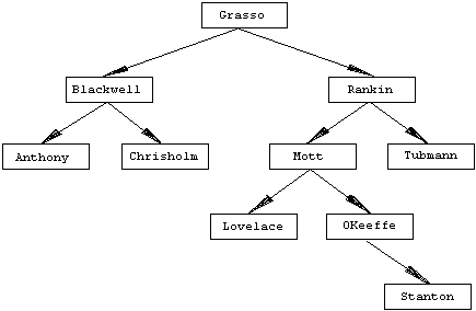
the right subtree, they follow it. Figure 6.3 shows an
example. Note that the same names, added in a different order, would produce a
somewhat different tree. Notice also that, although there are ten names in the
tree, you can find any of them in--at most--five steps.

Figure 6.3: Binary Search Tree
Every time you look at a cell in a binary
search tree during a search, you eliminate half the remaining cells from
consideration, and the search proceeds very quickly. If the size of the tree
were doubled, then, typically, only one extra step would be needed to search
it.
The time taken to find an
item in a binary search tree is, on the average, proportional to log2 N (or, in
fact, proportional to log N with logarithms to any base).
To build the tree, you start with an empty tree
and add items one by one. The procedure for adding an item is the same as for
finding one: you simply search for the place where it ought to be, and insert
it there. The algorithm is as follows:
If the current node is an empty tree, insert the item there.
Otherwise, compare the item to be inserted and the item stored in
the current node. Insert the item into the left subtree or the right subtree,
depending on the result of the comparison.
In Prolog, this requires three clauses, one for
each situation. The first clause is
insert(NewItem, empty,
tree(NewItem, empty, empty) :- !.
Translated to natural language, this code says
"The result of inserting NewItem
into empty is tree(NewItem, empty, empty)." The cut ensures that, if this clause can be used
successfully, no other clauses will be tried.
The second and third clauses take care of
insertion into nonempty trees:
insert(NewItem, tree(Element, Left, Right),
tree(Element, NewLeft, Right) :-
NewItem < Element,
!,
insert(NewItem, Left,
NewLeft).
insert(NewItem, tree(Element, Left, Right),
tree(Element, Left, NewRight) :-
insert(NewItem, Right,
NewRight).
If NewItem
< Element, you insert it into the
left subtree; otherwise, you insert it into the right subtree. Notice that,
because of the cuts, you get to the third clause only if neither of the
preceding clauses has succeeded. Also notice how much of the work is done by
matching arguments in the head of the rule.
(1) Tree-Based Sorting
Once
you have built the tree, it is easy to retrieve all the items in alphabetical
order. The algorithm is again a variant of depth-first search:
If the tree is empty, do nothing.
Otherwise, retrieve all the items in the left subtree, then the
current element, then all the items in the right subtree.
Or, in Prolog:
retrieve_all(empty). /*
Do nothing */
retrieve_all(tree(Item, Left, Right)) :-
retrieve_all(Left),
do_something_to(Item),
retrieve_all(Right).
You can sort a sequence of items by inserting
them into a tree and then retrieving them in order. For N items, this takes time proportional to N log N, because both
insertion and retrieval take time proportional to log N, and each of them has to be done N times. This is the fastest known sorting algorithm.
(2) Example
Program 11 uses this technique to alphabetize
character input. In this example we use some of Visual Prolog's standard predicates we haven't introduced before.
These predicates will be discussed in detail in later chapters.
/* Program ch06e11.pro */
DOMAINS
chartree = tree(char,
chartree, chartree); end
PREDICATES
nondeterm
do(chartree)
action(char,
chartree, chartree)
create_tree(chartree,
chartree)
insert(char,
chartree, chartree)
write_tree(chartree)
nondeterm repeat
CLAUSES
do(Tree):-
repeat,nl,
write("*****************************************************"),nl,
write("Enter 1 to
update tree\n"),
write("Enter 2 to show
tree\n"),
write("Enter 7 to
exit\n"),
write("*****************************************************"),nl,
write("Enter number -
"),
readchar(X),nl,
action(X, Tree, NewTree),
do(NewTree).
action('1',Tree,NewTree):-
write("Enter
characters or # to end: "),
create_Tree(Tree, NewTree).
action('2',Tree,Tree):-
write_Tree(Tree),
write("\nPress a key
to continue"),
readchar(_),nl.
action('7',
_, end):-
exit.
create_Tree(Tree,
NewTree):-
readchar(C),
C<>'#',!,
write(C, " "),
insert(C, Tree, TempTree),
create_Tree(TempTree,
NewTree).
create_Tree(Tree, Tree).
insert(New,end,tree(New,end,end)):-!.
insert(New,tree(Element,Left,Right),tree(Element,NewLeft,Right)):-
New<Element,!,
insert(New,Left,NewLeft).
insert(New,tree(Element,Left,Right),tree(Element,Left,NewRight)):-
insert(New,Right,NewRight).
write_Tree(end).
write_Tree(tree(Item,Left,Right)):-
write_Tree(Left),
write(Item, " "),
write_Tree(Right).
repeat.
repeat:-repeat.
GOAL
write("***************
Character tree sort *******************"),nl,
do(end).
Load and run Program 11 and watch how Visual Prolog does tree-based sorting on a
sequence of characters.
Exercises
Program 12 is similar to 11, but more complex. It uses the same
sorting technique to alphabetize any standard text file, line by line.
Typically it's more than five times faster than "SORT.EXE", the sort
program provided by DOS and OS/2, but it's beaten by the highly optimized
"sort" on UNIX. Nevertheless, tree-based sorting is remarkably
efficient.
In
this example we use some of the predicates from Visual Prolog's file system, to give you a taste of file
redirection. To redirect input or output to a file, you must tell the system
about the file; you use openread to
read from the file or openwrite
to write to it. Once files are open, you can switch I/O between an open file
and the screen with writedevice, and between an open file and the keyboard with readdevice. These
predicates are discussed in detail later in chapter 12.
Load and run Program 12.
When it prompts File to read type in the name of an existing text file; the
program will then alphabetize that file, line by line.
/* Program ch06e12.pro */
DOMAINS
treetype
= tree(string, treetype, treetype) ; empty
file = infile ; outfile
PREDICATES
main
read_input(treetype)
read_input_aux(treetype,
treetype)
insert(string,
treetype, treetype)
write_output(treetype)
CLAUSES
main
:-
write("PDC Prolog
Treesort"),nl,
write("File to
read: "),
readln(In),nl,
openread(infile, In), /* open the specified file for reading */
write("File to write:
"),
readln(Out),nl,
openwrite(outfile, Out),
readdevice(infile),
/*
redirect all read operations to the opened file */
read_input(Tree),
writedevice(outfile),
/*
redirect all write operations to the opened file */
write_output(Tree),
closefile(infile), /* close the file
opened for reading */
closefile(outfile).
/* * *
* * * * * * * * * * * * * * * * * * * * * * * * * * * * * * * * *
* read_input(Tree)
*
* reads lines from the current input device until EOF,
then *
* instantiates Tree to the binary search tree built
*
* therefrom
*
* * * * * * * * * * * * * * * * * * * * * * * * * * * * * * *
* * * * * /
read_input(Tree):-
read_input_aux(empty,Tree).
/* * *
* * * * * * * * * * * * * * * * * * * * * * * * * * * * * * *
* read_input_aux(Tree, NewTree)
*
*
reads a line, inserts it into Tree giving NewTree, *
*
and calls itself recursively unless at EOF. *
* * * * * * * * * * * * * * * * * * * * * * * * * * * * * * *
* * */
read_input_aux(Tree,
NewTree):-
readln(S),
!,
insert(S, Tree, Tree1),
read_input_aux(Tree1,
NewTree).
read_input_aux(Tree, Tree).
/* The first clause fails at EOF. */
/* * *
* * * * * * * * * * * * * * * * * * * * * * * * * * * * *
*
insert(Element, Tree, NewTree) *
* inserts Element into Tree giving
NewTree.
*
* * * * * * * * * * * * * * * * * * * * * * * * * * * * * * *
*/
insert(NewItem, empty,
tree(NewItem,empty,empty)):-!.
insert(NewItem,tree(Element,Left,Right),tree(Element,NewLeft,
Right)):-
NewItem < Element,
!,
insert(NewItem, Left,
NewLeft).
insert(NewItem,tree(Element,Left,Right),tree(Element,Left,NewRight)):-
insert(NewItem, Right,
NewRight).
/* * *
* * * * * * * * * * * * * * * * * * * * * * * * * * * * * * * *
* write_output(Tree)
*
* writes out the elements of Tree in alphabetical
order. *
* * * * * * * * * * * * * * * * * * * * * * * * * * * * * * *
* * * */
write_output(empty). /* Do
nothing */
write_output(tree(Item,Left,Right)):-
write_output(Left),
write(Item), nl,
write_output(Right).
GOAL
main,nl.
Use recursive data structures to implement hypertext. A hypertext is a structure in which each entry, made
up of several lines of text, is accompanied by pointers to several other
entries. Any entry can be connected to any other entry; for instance, you could
get to an entry about Abraham Lincoln either from "Presidents" or from
"Civil War."
